QC of Read Data
Learning Objectives:
- Understand how the FastQ format encodes quality
- Be able to evaluate a FastQC report
- Use Trimmommatic to clean FastQ reads
- Use a For loop to automate operations on multiple files
Bioinformatics workflows
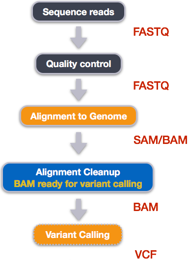
When working with high-throughput sequencing data, the raw reads you get off of the sequencer will need to pass through a number of different tools in order to generate your final desired output. The execution of this set of tools in a specified order is commonly referred to as a workflow or a pipeline.
An example of the workflow we will be using for our variant calling analysis is provided below with a brief description of each step.

- Quality control - Assessing quality using FastQC
- Quality control - Trimming and/or filtering reads (if necessary)
- Align reads to reference genome
- Perform post-alignment clean-up
- Variant calling
These workflows in bioinformatics adopt a plug-and-play approach in that the output of one tool can be easily used as input to another tool without any extensive configuration. Having standards for data formats is what makes this feasible. Standards ensure that data is stored in a way that is generally accepted and agreed upon within the community. The tools that are used to analyze data at different stages of the workflow are therefore built under the assumption that the data will be provided in a specific format.
Quality Control
The first step in the variant calling work flow is to take the FASTQ files received from the sequencing facility and assess the quality of the sequence reads.

Details on the FASTQ format
Although it looks complicated (and maybe it is), its easy to understand the fastq format with a little decoding. Some rules about the format include...
| Line | Description |
|---|---|
| 1 | Always begins with '@' and then information about the read |
| 2 | The actual DNA sequence |
| 3 | Always begins with a '+' and sometimes the same info in line 1 |
| 4 | Has a string of characters which represent the quality scores; must have same number of characters as line 2 |
so for example in our data set, one complete read is:
$ head -n4 SRR098281.fastq
@SRR098281.1 HWUSI-EAS1599_1:2:1:0:318 length=35
CNNNNNNNNNNNNNNNNNNNNNNNNNNNNNNNNNN
+SRR098281.1 HWUSI-EAS1599_1:2:1:0:318 length=35
#!!!!!!!!!!!!!!!!!!!!!!!!!!!!!!!!!!
This is a pretty bad read.
Notice that line 4 is:
#!!!!!!!!!!!!!!!!!!!!!!!!!!!!!!!!!!
As mentioned above, line 4 is a encoding of the quality. In this case, the code is the ASCII character table. According to the chart a '#' has the value 35 and '!' has the value 33 - But these values are not actually the quality scores! There are actually several historical differences in how Illumina and other players have encoded the scores. Heres the chart from wikipedia:
  SSSSSSSSSSSSSSSSSSSSSSSSSSSSSSSSSSSSSSSSS.....................................................
  ..........................XXXXXXXXXXXXXXXXXXXXXXXXXXXXXXXXXXXXXXXXXXXXXX......................
  ...............................IIIIIIIIIIIIIIIIIIIIIIIIIIIIIIIIIIIIIIIII......................
  .................................JJJJJJJJJJJJJJJJJJJJJJJJJJJJJJJJJJJJJJJ......................
  LLLLLLLLLLLLLLLLLLLLLLLLLLLLLLLLLLLLLLLLLL....................................................
  !"#$%&'()*+,-./0123456789:;<=>?@ABCDEFGHIJKLMNOPQRSTUVWXYZ[\]^_`abcdefghijklmnopqrstuvwxyz{|}~
  |                         |    |        |                              |                     |
 33                        59   64       73                            104                   126
  0........................26...31.......40
                           -5....0........9.............................40
                                 0........9.............................40
                                    3.....9.............................40
  0.2......................26...31........41

 S - Sanger        Phred+33,  raw reads typically (0, 40)
 X - Solexa        Solexa+64, raw reads typically (-5, 40)
 I - Illumina 1.3+ Phred+64,  raw reads typically (0, 40)
 J - Illumina 1.5+ Phred+64,  raw reads typically (3, 40)
     with 0=unused, 1=unused, 2=Read Segment Quality Control Indicator (bold)
     (Note: See discussion above).
 L - Illumina 1.8+ Phred+33,  raw reads typically (0, 41)
So using the Illumina 1.8 encoding, which is what you will mostly see from now on, our first c is called with a Phred score of 0 and our Ns are called with a score of 2. Read quality is assessed using the Phred Quality Score. This score is logarithmically based and the score values can be interpreted as follows:
| Phred Quality Score | Probability of incorrect base call | Base call accuracy |
|---|---|---|
| 10 | 1 in 10 | 90% |
| 20 | 1 in 100 | 99% |
| 30 | 1 in 1000 | 99.9% |
| 40 | 1 in 10,000 | 99.99% |
| 50 | 1 in 100,000 | 99.999% |
| 60 | 1 in 1,000,000 | 99.9999% |
Let's use the following read as an example:
@HWI-ST330:304:H045HADXX:1:1101:1111:61397
CACTTGTAAGGGCAGGCCCCCTTCACCCTCCCGCTCCTGGGGGANNNNNNNNNNANNNCGAGGCCCTGGGGTAGAGGGNNNNNNNNNNNNNNGATCTTGG
+
@?@DDDDDDHHH?GH:?FCBGGB@C?DBEGIIIIAEF;FCGGI#########################################################
As mentioned previously, line 4 has characters encoding the quality of each nucleotide in the read. The legend below provides the mapping of quality scores (Phred-33) to the quality encoding characters. ** Different quality encoding scales exist (differing by offset in the ASCII table), but note the most commonly used one is fastqsanger **
 Quality encoding: !"#$%&'()*+,-./0123456789:;<=>?@ABCDEFGHI
                   |         |         |         |         |
    Quality score: 0........10........20........30........40
Using the quality encoding character legend, the first nucleotide in the read (C) is called with a quality score of 31 and our Ns are called with a score of 2. As you can tell by now, this is a bad read.
Each quality score represents the probability that the corresponding nucleotide call is incorrect. This quality score is logarithmically based and is calculated as:
Q = -10 x log10(P), where P is the probability that a base call is erroneous
These probability values are the results from the base calling algorithm and dependent on how much signal was captured for the base incorporation.
FastQC
FastQC (http://www.bioinformatics.babraham.ac.uk/projects/fastqc/) provides a simple way to do some quality control checks on raw sequence data coming from high throughput sequencing pipelines. It provides a modular set of analyses which you can use to give a quick impression of whether your data has any problems of which you should be aware before doing any further analysis.
The main functions of FastQC are:
- Import of data from BAM, SAM or FastQ files (any variant)
- Providing a quick overview to tell you in which areas there may be problems
- Summary graphs and tables to quickly assess your data
- Export of results to an HTML based permanent report
- Offline operation to allow automated generation of reports without running the interactive application
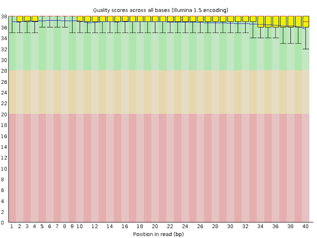
Rather than looking at quality scores for each individual read, FastQC looks at quality collectively across all reads within a sample. The image below is a plot that indicates a (very) good quality sample:

On the x-axis you have the base position in the read, and on the y-axis you have quality scores. In this example, the sample contains reads that are 40 bp long. For each position, there is a box plotted to illustrate the distribution of values (with the whiskers indicating the 90th and 10th percentile scores). For every position here, the quality values do not drop much lower than 32 -- which if you refer to the table above is a pretty good quality score. The plot background is also color-coded to identify good (green), acceptable (yellow), and bad (red) quality scores.
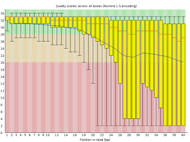
Now let's take a look at a quality plot on the other end of the spectrum.

Here, we see positions within the read in which the boxes span a much wider range. Also, quality scores drop quite low into the 'bad' range, particularly on the tail end of the reads. When you encounter a quality plot such as this one, the first step is to troubleshoot. Why might we be seeing something like this?
The FASTQC tool produces several other diagnostic plots to assess sample quality, in addition to the one plotted above.
Running FASTQC
A. Stage your data
Create a working directory for your analysis
$ cd
# this command takes us to the home directory

$ mkdir dc_workshop
Create three three subdirectories
mkdir dc_workshop/data
mkdir dc_workshop/docs
mkdir dc_workshop/results
The sample data we will be working with is in a hidden directory (placing a '.' in front of a directory name hides the directory. In the next step we will move some of those hidden files into our new dirctories to start our project.
Move our sample data to our working (home) directory
$ mv ~/.dc_sampledata_lite/untrimmed_fastq/ ~/dc_workshop/data/
B. Run FastQC
Navigate to the initial fastq dataset
$ cd ~/dc_workshop/data/untrimmed_fastq/To run the fastqc program, we call it from its location in
~/FastQC. fastqc will accept multiple file names as input, so we can use the *.fastq wildcard.Run FastQC on all fastq files in the directory
$ ~/FastQC/fastqc *.fastqNow, let's create a home for our results
$ mkdir ~/dc_workshop/results/fastqc_untrimmed_readsNext, move the files there (recall, we are still in
~/dc_workshop/data/untrimmed_fastq/)$ mv *.zip ~/dc_workshop/results/fastqc_untrimmed_reads/ $ mv *.html ~/dc_workshop/results/fastqc_untrimmed_reads/
C. Results
Lets examine the results in detail
Navigate to the results and view the directory contents
$ cd ~/dc_workshop/results/fastqc_untrimmed_reads/
$ ls
The zip files need to be unpacked with the 'unzip' program.
Use unzip to unzip the FastQC results:
$ unzip *.zipDid it work? No, because 'unzip' expects to get only one zip file. Welcome to the real world. We could do each file, one by one, but what if we have 500 files? There is a smarter way. We can save time by using a simple shell 'for loop' to iterate through the list of files in *.zip. After you type the first line, you will get a special '>' prompt to type next next lines. You start with 'do', then enter your commands, then end with 'done' to execute the loop.
Build a
forloop to unzip the files$ for zip in *.zip > do > unzip $zip > doneNote that, in the first line, we create a variable named 'zip'. After that, we call that variable with the syntax $zip. $zip is assigned the value of each item (file) in the list *.zip, once for each iteration of the loop.
This loop is basically a simple program. When it runs, it will run unzip once for each file (whose name is stored in the $zip variable). The contents of each file will be unpacked into a separate directory by the unzip program.
The for loop is interpreted as a multipart command. If you press the up arrow on your keyboard to recall the command, it will be shown like so:
$ for zip in *.zip; do echo File $zip; unzip $zip; done
When you check your history later, it will help your remember what you did!
D. Document your work
To save a record, let's cat all fastqc summary.txts into one fullreport.txt and move this to ``~/dcworkshop/docs``. You can use wildcards in paths as well as file names. Do you remember how we said 'cat' is really meant for concatenating text files?
cat */summary.txt > ~/dc_workshop/docs/fastqc_summaries.txt
How to clean reads using Trimmomatic
A detailed explanation of features
Once we have an idea of the quality of our raw data, it is time to trim away adapters and filter out poor quality score reads. To accomplish this task we will use Trimmomatic http://www.usadellab.org/cms/?page=trimmomatic.
Trimmomatic is a java based program that can remove sequencer specific reads and nucleotides that fall below a certain threshold. Trimmomatic can be multithreaded to run quickly.
Because Trimmomatic is java based, it is run using the command:
java jar trimmomatic-0.32.jar
What follows this are the specific commands that tells the program exactly how you want it to operate. Trimmomatic has a variety of options and parameters:
- -threds How many processors do you want Trimmomatic to run with?
- SE or PE Single End or Paired End reads?
- -phred33 or -phred64 Which quality score do your reads have?
- SLIDINGWINDOW Perform sliding window trimming, cutting once the average quality within the window falls below a threshold.
- LEADING Cut bases off the start of a read, if below a threshold quality.
- TRAILING Cut bases off the end of a read, if below a threshold quality.
- CROP Cut the read to a specified length.
- HEADCROP Cut the specified number of bases from the start of the read.
- MINLEN Drop an entire read if it is below a specified length.
- TOPHRED33 Convert quality scores to Phred-33.
- TOPHRED64 Convert quality scores to Phred-64.
A generic command for Trimmomatic looks like this:
java jar trimmomatic-0.32.jar SE -thr
A complete command for Trimmomatic will look something like this:
java jar trimmomatic-0.32.jar SE -threads 4 -phred64 SRR1056.fastq SRR1056trimmed.fastq ILLUMINACLIP:SRRadapters.fa SLIDINGWINDOW:4:20
This command tells Trimmomatic to run on a Single End file (SRR_0156.fastq, in this case), the output file will be called SRR_0156_trimmed.fastq, there is a file with Illumina adapters called SRR_adapters.fa, and we are using a sliding window of size 4 that will remove those bases if their phred score is below 20.
Exercise - Running Trimmomatic
Go to the untrimmed fastq data location:
$ cd /home/dcuser/dc_workshop/data/untrimmed_fastq
The command line incantation for trimmomatic is more complicated. This is where what you have been learning about accessing your command line history will start to become important.
The general form of the command is:
java -jar ~/Trimmomatic-0.32/trimmomatic-0.32.jar inputfile outputfile OPTION:VALUE...
'java -jar' calls the Java program, which is needed to run trimmomargumentstic, which lived in a 'jar' file (trimmomatic-0.32.jar), a special kind of java archive that is often used for programs written in the Java programing language. If you see a new program that ends in '.jar', you will know it is a java program that is executed 'java -jar program name'. The 'SE' argument is a keyword that specifies we are working with single-end reads.
The next two arguments are input file and output file names. These are then followed by a series of options. The specifics of how options are passed to a program are different depending on the program. You will always have to read the manual of a new program to learn which way it expects its command-line arguments to be composed.
So, for the single fastq input file 'SRR098283.fastq', the command would be:
$ java -jar /home/dcuser/Trimmomatic-0.32/trimmomatic-0.32.jar SE SRR098283.fastq \
SRR098283.fastq_trim.fastq SLIDINGWINDOW:4:20 MINLEN:20

TrimmomaticSE: Started with arguments: SRR098283.fastq SRR098283.fastq_trim.fastq SLIDINGWINDOW:4:20 MINLEN:20
Automatically using 2 threads
Quality encoding detected as phred33
Input Reads: 21564058 Surviving: 17030985 (78.98%) Dropped: 4533073 (21.02%)
TrimmomaticSE: Completed successfully
So that worked and we have a new fastq file.
$ ls SRR098283*
SRR098283.fastq  SRR098283.fastq_trim.fastq
Now we know how to run trimmomatic but there is some good news and bad news.
One should always ask for the bad news first. Trimmomatic only operates on
one input file at a time and we have more than one input file. The good news?
We already know how to use a for loop to deal with this situation.
    $ for infile in *.fastq
    >do
    >outfile=$infile\_trim.fastq
    >java -jar ~/Trimmomatic-0.32/trimmomatic-0.32.jar SE $infile $outfile SLIDINGWINDOW:4:20 MINLEN:20
    >done
Do you remember how the first specifies a variable that is assigned the value of each item in the list in turn? We can call it whatever we like. This time it is called infile. Note that the third line of this for loop is creating a second variable called outfile. We assign it the value of $infile with '_trim.fastq' appended to it. The '\' escape character is used so the shell knows that whatever follows \ is not part of the variable name $infile. There are no spaces before or after the '='.
