Automating with Shell Scripting

Learning Objectives:

Understand what a shell script is
Learn how automate an analytical workflow
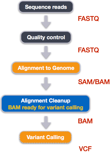
Understand the different steps involved in variant calling
Use a series of command line tools to execute a variant calling workflow
Becoming familiar with data formats encountered during variant calling

What is a shell script?

A shell script is basically a text file that contains a list of commands that are executed sequentially. The commands in a shell script are the same as you would use on the command line.

Once you have worked out the details and tested your commands in the shell, you can save them into a file so, the next time, you can automate the process with a script.

The basic anatomy of a shell script is a file with a list of commands. That is also the definition of pretty much any computer program.

#!/bin/bash

cd ~/dc_sample_data

for file in untrimmed_fastq/*.fastq
do
  echo "My file name is $file"
done

This looks a lot like the for loops we saw earlier. In fact, it is no different, apart from using indentation and the lack of the '>' prompts; it's just saved in a text file. The line at the top ('#!/bin/bash') is commonly called the shebang line, which is a special kind of comment that tells the shell which program is to be used as the 'intepreter' that executes the code.

In this case, the interpreter is bash, which is the shell environment we are working in. The same approach is also used for other scripting languages such as perl and python.

How to run a shell script

There are two ways to run a shell script the first way is to specify the interpreter (bash) and the name of the script. By convention, shell script use the .sh extension, though this is not enforced.

$ bash myscript.sh
My file name is untrimmed_fastq/SRR097977.fastq
My file name is untrimmed_fastq/SRR098026.fastq

The second was is a little more complicated to set up.

The first step, which only needs to be done once, is to modify the file 'permissions' of the text file so that the shell knows the file is executable.

$ chmod +x myscript.sh

After that, you can run the script as a regular program by just typing it's name on the command line.

$ ./myscript.sh
My file name is untrimmed_fastq/SRR097977.fastq
My file name is untrimmed_fastq/SRR098026.fastq

The thing about running programs on the command line is that the shell may not know the location of your executables unless they are in the 'path' of know locations for programs. So, you need to tell the shell the path to your script, which is './' if it is in the same directory.

Exercise 1) Use nano to save the code above to a script called myscript.sh 2) run the script

A real shell script

Now, let's do something real. First, recall the code from our our fastqc workflow from this morning, with a few extra "echo" statements.

cd ~/dc_workshop/data/untrimmed_fastq/

echo "Running fastqc..."
~/FastQC/fastqc *.fastq
mkdir -p ~/dc_workshop/results/fastqc_untrimmed_reads

echo "saving..."
mv *.zip ~/dc_workshop/results/fastqc_untrimmed_reads/
mv *.html ~/dc_workshop/results/fastqc_untrimmed_reads/

cd ~/dc_workshop/results/fastqc_untrimmed_reads/

echo "Unzipping..."
for zip in *.zip
do
  unzip $zip
done

echo "saving..."
cat */summary.txt > ~/dc_workshop/docs/fastqc_summaries.txt

Exercise

1) Use nano to create a shell script using with the code above (you can copy/paste), named read_qc.sh

2) Run the script

3) Bonus points: Use something you learned yesterday to save the output of the script to a file while it is running.

Setting up

To get started with this lesson, make sure you are in dc_workshop. Now let's copy over the reference data required for alignment:

$ cd ~/dc_workshop
$ cp -r ~/.dc_sampledata_lite/ref_genome/ data/

Your directory structure should now look like this:

dc_workshop
├── data
    ├── ref_genome
        └── ecoli_rel606.fasta
    ├── untrimmed_fastq
    └── trimmed_fastq
        ├── SRR097977.fastq
        ├── SRR098026.fastq
        ├── SRR098027.fastq
        ├── SRR098028.fastq
        ├── SRR098281.fastq
        └── SRR098283.fastq
 ├── results
 └── docs

You will also need to create directories for the results that will be generated as part of the workflow:

$ mkdir  results/sai results/sam results/bam results/bcf results/vcf

NOTE: All of the tools that we will be using in this workflow have been pre-installed on our remote computer

Alignment to a reference genome

We have already trimmed our reads so now the next step is alignment of our quality reads to the reference genome.

workflow_align

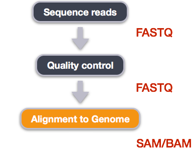
We perform read alignment or mapping to determine where in the genome our reads originated from. There are a number of tools to choose from and while there is no gold standard there are some tools that are better suited for particular NGS analyses. We will be using the Burrows Wheeler Aligner (BWA), which is a software package for mapping low-divergent sequences against a large reference genome. The alignment process consists of two steps:

Indexing the reference genome
Aligning the reads to the reference genome

Index the reference genome

Our first step is to index the reference genome for use by BWA. NOTE: This only has to be run once. The only reason you would want to create a new index is if you are working with a different reference genome or you are using a different tool for alignment.

$ bwa index data/ref_genome/ecoli_rel606.fasta     # This step helps with the speed of alignment

Eventually we will loop over all of our files to run this workflow on all of our samples, but for now we're going to work on just one sample in our dataset SRR098283.fastq:

$ ls -alh ~/dc_workshop/data/trimmed_fastq/SRR097977.fastq_trim.fastq

Align reads to reference genome

The alignment process consists of choosing an appropriate reference genome to map our reads against and then deciding on an aligner. BWA consists of three algorithms: BWA-backtrack, BWA-SW and BWA-MEM. The first algorithm is designed for Illumina sequence reads up to 100bp, while the rest two for longer sequences ranged from 70bp to 1Mbp. BWA-MEM and BWA-SW share similar features such as long-read support and split alignment, but BWA-MEM, which is the latest, is generally recommended for high-quality queries as it is faster and more accurate.

Since we are working with short reads we will be using BWA-backtrack. The usage for BWA-backtrack is

$ bwa aln path/to/ref_genome.fasta path/to/fastq > SAIfile

This will create a .sai file which is an intermediate file containing the suffix array indexes.

Have a look at the bwa options page. While we are running bwa with the default parameters here, your use case might require a change of parameters. NOTE: Always read the manual page for any tool before using and try to understand the options.

$ bwa aln data/ref_genome/ecoli_rel606.fasta \
    data/trimmed_fastq/SRR097977.fastq_trim.fastq > results/sai/SRR097977.aligned.sai

Alignment cleanup

workflow_clean

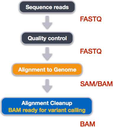
Post-alignment processing of the alignment file includes:

Converting output SAI alignment file to a BAM file
Sorting the BAM file by coordinate

Convert the format of the alignment to SAM/BAM

The SAI file is not a standard alignment output file and will need to be converted into a SAM file before we can do any downstream processing.

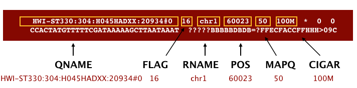
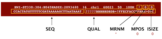
SAM/BAM format

The SAM file, is a tab-delimited text file that contains information for each individual read and its alignment to the genome. While we do not have time to go in detail of the features of the SAM format, the paper by Heng Li et al. provides a lot more detail on the specification. The binary version of SAM is called a BAM file.

The file begins with a header, which is optional. The header is used to describe source of data, reference sequence, method of alignment, etc., this will change depending on the aligner being used. Following the header is the alignment section. Each line that follows corresponds to alignment information for a single read. Each alignment line has 11 mandatory fields for essential mapping information and a variable number of other fields for aligner specific information. An example entry from a SAM file is displayed below with the different fields highlighted.

sam_bam1

sam_bam2

First we will use the bwa samse command to convert the .sai file to SAM format:

$ bwa samse data/ref_genome/ecoli_rel606.fasta \
      results/sai/SRR097977.aligned.sai \
      data/trimmed_fastq/SRR097977.fastq_trim.fastq > \
      results/sam/SRR097977.aligned.sam

Explore the information within your SAM file:

$ head results/sam/SRR097977.aligned.sam

Now convert the SAM file to BAM format for use by downstream tools:

$ samtools view -S -b results/sam/SRR097977.aligned.sam > results/bam/SRR097977.aligned.bam

Sort BAM file by coordinates

Sort the BAM file:

$ samtools sort results/bam/SRR097977.aligned.bam results/bam/SRR097977.aligned.sorted

SAM/BAM files can be sorted in multiple ways, e.g. by location of alignment on the chromosome, by read name, etc. It is important to be aware that different alignment tools will output differently sorted SAM/BAM, and different downstream tools require differently sorted alignment files as input.

Variant calling

A variant call is a conclusion that there is a nucleotide difference vs. some reference at a given position in an individual genome or transcriptome, often referred to as a Single Nucleotide Polymorphism (SNP). The call is usually accompanied by an estimate of variant frequency and some measure of confidence. Similar to other steps in this workflow, there are number of tools available for variant calling. In this workshop we will be using bcftools, but there are a few things we need to do before actually calling the variants.

workflow

Step 1: Calculate the read coverage of positions in the genome

Do the first pass on variant calling by counting read coverage with samtools mpileup:

$ samtools mpileup -g -f data/ref_genome/ecoli_rel606.fasta \
            results/bam/SRR097977.aligned.sorted.bam > results/bcf/SRR097977_raw.bcf

We have only generated a file with coverage information for every base with the above command; to actually identify variants, we have to use a different tool from the samtools suite called bcftools.

Step 2: Detect the single nucleotide polymorphisms (SNPs)

Identify SNPs using bcftools:

$ bcftools view -bvcg results/bcf/SRR097977_raw.bcf > results/bcf/SRR097977_variants.bcf

Step 3: Filter and report the SNP variants in VCF (variant calling format)

Filter the SNPs for the final output in VCF format, using vcfutils.pl:

$ bcftools view results/bcf/SRR097977_variants.bcf \ | /usr/share/samtools/vcfutils.pl varFilter - > results/vcf/SRR097977_final_variants.vcf

bcftools view converts the binary format of bcf files into human readable format (tab-delimited) for vcfutils.pl to perform the filtering. Note that the output is in VCF format, which is a text format.

Explore the VCF format:

$ less results/vcf/SRR097977_final_variants.vcf

You will see the header which describes the format, when the file was created, the tools version along with the command line parameters used and some additional column information:

##reference=file://data/ref_genome/ecoli_rel606.fasta
##contig=<ID=NC_012967.1,length=4629812>
##ALT=<ID=X,Description="Represents allele(s) other than observed.">
##INFO=<ID=INDEL,Number=0,Type=Flag,Description="Indicates that the variant is an INDEL.">
##INFO=<ID=IDV,Number=1,Type=Integer,Description="Maximum number of reads supporting an indel">
##INFO=<ID=IMF,Number=1,Type=Float,Description="Maximum fraction of reads supporting an indel">
##INFO=<ID=DP,Number=1,Type=Integer,Description="Raw read depth">
.
.
.
.
##FORMAT=<ID=GT,Number=1,Type=String,Description="Genotype">
##FORMAT=<ID=GQ,Number=1,Type=Integer,Description="Genotype Quality">
##FORMAT=<ID=GL,Number=3,Type=Float,Description="Likelihoods for RR,RA,AA genotypes (R=ref,A=alt)">
##FORMAT=<ID=DP,Number=1,Type=Integer,Description="# high-quality bases">
##FORMAT=<ID=DV,Number=1,Type=Integer,Description="# high-quality non-reference bases">
##FORMAT=<ID=SP,Number=1,Type=Integer,Description="Phred-scaled strand bias P-value">
##FORMAT=<ID=PL,Number=G,Type=Integer,Description="List of Phred-scaled genotype likelihoods">

Followed by the variant information:

#CHROM  POS     ID      REF     ALT     QUAL    FILTER  INFO    FORMAT  results/bam/SRR097977.aligned.sorted.bam
NC_012967.1     9972    .       T       G       222     .       DP=28;VDB=8.911920e-02;AF1=1;AC1=2;DP4=0,0,19,7;MQ=36;FQ=-105   GT:PL:GQ        1/1:255,78,0:99
NC_012967.1     10563   .       G       A       222     .       DP=27;VDB=6.399241e-02;AF1=1;AC1=2;DP4=0,0,8,18;MQ=36;FQ=-105   GT:PL:GQ        1/1:255,78,0:99
NC_012967.1     81158   .       A       C       222     .       DP=37;VDB=2.579489e-02;AF1=1;AC1=2;DP4=0,0,15,21;MQ=37;FQ=-135  GT:PL:GQ        1/1:255,108,0:99
NC_012967.1     216480  .       C       T       222     .       DP=39;VDB=2.356774e-01;AF1=1;AC1=2;DP4=0,0,19,17;MQ=36;FQ=-135  GT:PL:GQ        1/1:255,108,0:99
NC_012967.1     247796  .       T       C       221     .       DP=18;VDB=1.887634e-01;AF1=1;AC1=2;DP4=0,0,7,11;MQ=35;FQ=-81    GT:PL:GQ        1/1:254,54,0:99

The first columns represent the information we have about a predicted variation.

CHROM and POS provide the config information and position where the variation occurs.

ID is a . until we add annotation information.

REF and ALT represent the genotype at the reference and in the sample, always on the foward strand.

QUAL then is the Phred scaled probablity that the observed variant exists at this site. Ideally you would need nothing else to filter out bad variant calls, but in reality we still need to filter on multiple other metrics.

The FILTER field is a ., i.e. no filter has been applied, otherwise it will be set to either PASS or show the (quality) filters this variant failed.

The last columns contains the genotypes and can be a bit more tricky to decode. In brief, we have:

GT: The genotype of this sample which for a diploid genome is encoded with a 0 for the REF allele, 1 for the first ALT allele, 2 for the second and so on. So 0/0 means homozygous reference, 0/1 is heterozygous, and 1/1 is homozygous for the alternate allele. For a diploid organism, the GT field indicates the two alleles carried by the sample, encoded by a 0 for the REF allele, 1 for the first ALT allele, 2 for the second ALT allele, etc.
GQ: the Phred-scaled confidence for the genotype
AD, DP: Reflect the depth per allele by sample and coverage
PL: the likelihoods of the given genotypes

The BROAD's VCF guide is an excellent place to learn more about VCF file format.

Assess the alignment (visualization) - optional step

In order for us to look at the alignment files in a genome browser, we will need to index the BAM file using samtools:

$ samtools index results/bam/SRR097977.aligned.sorted.bam

Transfer files to your laptop

Using FileZilla, transfer the following 4 files to your local machine:

results/bam/SRR097977.aligned.sorted.bam

results/bam/SRR097977.aligned.sorted.bam.bai

data/ref_genome/ecoli_rel606.fasta

results/vcf/SRR097977_final_variants.vcf

Visualize

Start IGV
Load the genome file into IGV using the "Load Genomes from File..." option under the "Genomes" pull-down menu.
Load the .bam file using the "Load from File..." option under the "File" pull-down menu. IGV requires the .bai file to be in the same location as the .bam file that is loaded into IGV, but there is no direct use for that file.
Load in the VCF file using the "Load from File..." option under the "File" pull-down menu

Your IGV browser should look like the screenshot below:

IGV

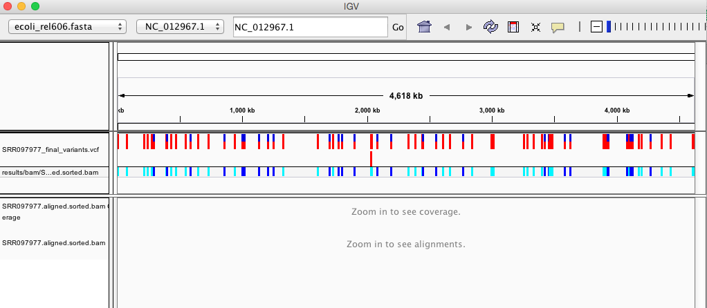
There should be two tracks: one coresponding to your BAM file and the other for your VCF file.

In the VCF track, each bar across the top of the plot shows the allele fraction for a single locus. The second bar will show the genotypes for each locus in each sample. We only have one sample called here so we only see a single line. Dark blue = heterozygous, Cyan = homozygous variant, Grey = reference. Filtered entries are transparent.

Zoom in to inspect variants you see in your filtered VCF file to become more familiar with IGV. See how quality information corresponds to alignment information at those loci.